The evolution of DNNs can be traced back to foundational work in the mid-20th century. However, significant advancements occurred in the 1980s with the introduction of backpropagation for training multi-layer networks.
The resurgence of interest in deep learning in the 2000s was fueled by increased computational power and large datasets, leading to breakthroughs in tasks like image and speech recognition.
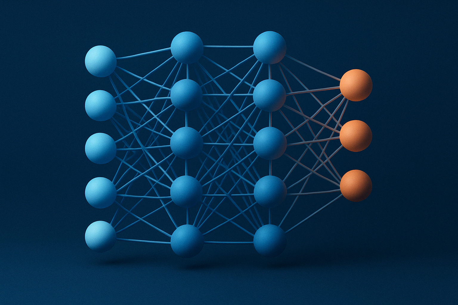
At their core, DNNs are artificial neural networks with multiple hidden layers between the input and output layers. This depth allows them to model complex, non-linear relationships in data, making them particularly effective for tasks that involve pattern recognition and data abstraction. Each layer in a DNN transforms its input data into a slightly more abstract and composite representation, facilitating the network’s ability to learn intricate features of the data.
A typical Artificial Neural Network (ANN) is composed of numerous interconnected processing units called neurons, each generating a stream of real-numbered activations.
The input neurons are activated through sensors that perceive the external environment, while other neurons receive signals via weighted links from previously activated neurons. Some neurons may also affect the environment directly by initiating actions.
The process of learning, or credit assignment, involves identifying the right set of connection weights that lead the network to exhibit the intended behavior, such as controlling a vehicle. Depending on the specific task and the architecture of the network, this behavior might rely on a sequence of interconnected processing steps, where each stage often applies a non-linear transformation to the accumulated activity from earlier layers. Deep learning focuses on effectively assigning credit across these multiple layers of computation.
In the 2000s, deep neural networks began to gain substantial attention by surpassing other machine learning techniques, like kernel-based methods, in many high-impact applications. Since 2009, supervised deep neural networks have won numerous international competitions in pattern recognition, even achieving superhuman performance in certain visual recognition tasks.
Additionally, deep neural networks have become increasingly important in reinforcement learning, a domain where guidance is provided not by explicit labels, but by interacting with and learning from the environment.
A neural network can be understood as a type of computational graph, where each node, or unit of computation, is a neuron. What makes neural networks significantly more powerful than the individual components is that their parameters are jointly learned, allowing the network to act as a highly optimized composite function. Additionally, the use of nonlinear activation functions between layers greatly enhances the network’s ability to represent complex patterns.
Training DNNs involves adjusting the weights of the network to minimize the difference between the predicted outputs and the actual targets. This process typically employs gradient-based optimization techniques, with backpropagation being the most common method for computing gradients.
This approach treats the entire neural network as a graph of connected operations. Imagine a chain of functions, where each step transforms data slightly, like filtering, combining, or reshaping it. When the network makes a prediction, data flows forward through these connected functions.
During backpropagation, the process reverses. The system traces each step backward and calculates how much each operation contributed to the final error. This method breaks complex computations into simple, local pieces, which makes it flexible and reusable.
It’s widely used in modern deep learning frameworks like TensorFlow and PyTorch, allowing developers to focus on building models without manually coding derivatives.
In this method, the focus is on the output values after each neuron’s activation function has been applied. These are the values the network uses to make decisions.
During learning, the model compares its predictions with the correct answers and calculates how far off it was. This error is then pushed backward through the network. At each layer, the model checks how much of that error is due to the specific output from the neuron, and uses that information to adjust the settings (or “weights”) that led to that output.
This perspective is helpful when you want to understand how the final predictions change in response to specific outputs at each step.
Here, attention is given to the raw input each neuron receives before its activation function is applied. This is useful because it lets us see how sensitive the network is to its internal state before making a decision.
By examining these pre-activation values, we can get a clearer picture of how the network transforms data and how errors flow backward through that transformation.
This method is often helpful in understanding how certain types of neurons (like those using the ReLU function) behave, especially when they shut off or remain inactive. It’s a valuable lens when analyzing the fine-tuned workings of the network’s internals.
This technique focuses on processing many neurons at once, using vector or matrix operations. Rather than looking at one neuron at a time, this method handles entire layers of neurons simultaneously. It’s particularly efficient for computer systems because it reduces the number of calculations and makes better use of hardware like GPUs.
When the network trains, the adjustments to the model are computed for whole groups of neurons in parallel. This approach is commonly used in real-world training environments where speed and scalability are crucial. It doesn’t change the theory of backpropagation, it just makes it much faster and easier to run on large models.
Training deep neural networks (DNNs) in supervised learning settings is often computationally intensive and demands large volumes of labeled data, a challenge that is only growing as DNNs become more complex.
Federated Learning (FL) presents a promising solution. In FL, multiple devices (clients) collaboratively train a shared machine learning model, typically a DNN, without ever sending their raw data to a central server. Instead, each device performs local training and only shares model updates (like gradients or parameters), allowing the global model to improve while keeping user data private and secure.
Distributed learning doesn’t change the math behind computational graphs, post-activation, or pre-activation backpropagation, it simply scales them.
In deep learning, overfitting happens when a neural network performs extremely well on its training data but fails to deliver accurate predictions on new, unseen examples. This occurs because the model ends up memorizing small, often random patterns or noise in the training data that do not generalize well to other inputs. In extreme cases, this behavior is known as memorization.
The opposite of overfitting is generalization,the ability of a model to make accurate predictions on data it has never encountered before. Generalization is the ultimate goal in machine learning.
There are two common signs of overfitting:
Regularization techniques add penalties to model complexity during training. By discouraging large weights, they help guide the model toward simpler, more generalizable solutions.
Combining the predictions of multiple models, or creating variation within a single model, as in the case of dropout, can reduce overfitting.
Dropout randomly disables parts of the network during training, forcing the model to learn redundant representations and act as an implicit ensemble.
Instead of training a model until it fully minimizes training error, early stopping monitors a validation set and halts training when performance on this separate data begins to degrade.
This prevents the model from over-specializing on the training set.
Layer-wise pretraining involves training each part of the network one at a time and using these trained parts to initialize the full network. This offers a good starting point and acts as an indirect regularizer, helping avoid poor local minima during training.
These strategies involve starting with a simpler version of the problem or network and gradually increasing complexity. Like pretraining, they guide the network toward more stable learning paths.
In domains like image and text processing, certain architectural assumptions (e.g., shared filters in CNNs or shared weights in RNNs) reduce the number of free parameters. This constraint lowers the risk of overfitting by simplifying the model’s structure based on domain knowledge.
One of the major challenges in training deep neural networks is the issue of vanishing and exploding gradients, which can severely hinder the learning process. These problems arise during backpropagation, where error signals are passed backward through the network to update weights.
In the case of vanishing gradients, the error signals shrink as they move through each layer, causing the early layers to receive almost no updates. This leads to slow or stalled learning in those layers. Conversely, with exploding gradients, the error signals grow exponentially as they are propagated, resulting in unstable weight updates and erratic training behavior.
These issues are especially common in very deep networks and recurrent neural networks (RNNs), where the repeated multiplication of gradients compounds the problem.
To address this, several solutions have been introduced. These include using activation functions like ReLU, which help maintain stronger gradient signals; gradient clipping, which caps the maximum size of gradients to prevent them from becoming too large; and the adoption of specialized architectures such as LSTMs for sequences and batch normalization, which stabilizes the training process by normalizing intermediate outputs.
Deep neural networks are highly complex and nonlinear, which makes them difficult to interpret or explain.
One major challenge stems from the multiscale and distributed nature of their internal representations: some neurons respond only to very specific inputs, while others influence a broader range of data. As a result, each prediction is shaped by a combination of local and global activations, making it hard to trace back the outcome to a simple, linear explanation.
Another issue arises from the depth of modern architectures, which can lead to what’s known as the “shattered gradient” problem, a phenomenon where gradients behave like random noise locally, reducing the reliability of gradient-based explanations.
Finally, a key limitation in current interpretability methods is the difficulty in identifying a reference input (or root point) that is both similar to the input being explained and free from adversarial artifacts.
Together, these factors contribute to the inherent instability and opacity of DNN decision-making.
This article explored the structure, functionality, and challenges of Deep Neural Networks (DNNs), one of the most powerful tools in modern artificial intelligence. Information presented here integrates insights from recent academic research to offer accurate, current perspectives.
We examined key architectural components, training strategies such as backpropagation, and issues like overfitting, vanishing gradients, and interpretability. We also discussed advanced techniques like dropout, regularization, and curriculum learning that help improve generalization and stability in DNNs.
As the field continues to evolve, DNNs remain central to breakthroughs in image recognition, natural language processing, and autonomous systems.
1LineCrypto © 2025 All rights reserved